Stanford UFLDL Tutorial Work Through (2) - Logistic Regression

|

Link to the tutorial: Unsupervised Feature Learning and Deep Learning: Logistic Regression

Problem

To illustrate logistic regression, let’s reuse the notation of the variables \(X\), \(\Theta\), and \(Y\) from section (1) for linear regression.

Different from linear regression, which is usually used to predict continuous output values, logistic regression is used in classification problems, which have discrete \(y\) outputs. For example, in a two class classification problem, the \(y\) output has two values, 0 and 1. In a logistic regression problem, we want to find a function \(H_{\Theta}\) such that \(H_{\Theta}(X)\) produces a output vector that matches as much as possible to the output variable \(Y\).

Sigmoid/Logistic Function

Before we derive the cost function of logistic regression, we need to introduce a convenient function called the sigmoid function, or logistic function if you like. The function is given by:

[S(z)=\frac{1}{1+e^{-z}}]

The sigmoid function has the following properties:

  • It is a “S” shape function bounded between 0 and 1. This is usefully because in the process of generating a binary output from \(H_{\Theta}(X)\), the sigmoid function is used to convert the output of a linear function, say \(Z = X\Theta\), into a probability that is used in calculate the cost. Please find the the graph of the sigmoid function below:
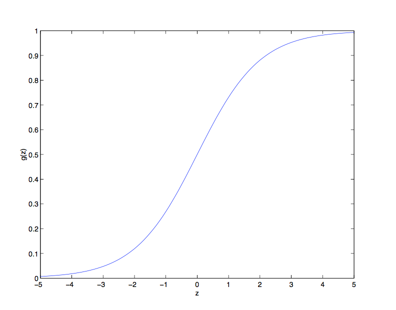
sigmoid

  • The derivative of the sigmoid function has a very nice form that makes logistic regression a very clean linear method. The derivative is given in the following:

[\begin{array}{ccl} S’(z)&=&\frac{d}{dz}\frac{1}{1+e^{-z}}
&=&\frac{e^{-z}}{(1+e^{-z})^2}
&=&\frac{1}{1+e^{-z}}\cdot\frac{1+e^{-z}-1}{1+e^{-z}}
&=&\frac{1}{1+e^{-z}}\cdot(1-\frac{1}{1+e^{-z}})
&=&S(z)(1-S(z)) \end{array}]

The maximum likelihood function \(\ell(\Theta)\)

Now we can define the following two functions to calculate the probabilities an input record belongs to a certain class:

[\begin{array}{l} P(y=1|x^{(i)})=h_{\Theta}(x^{(i)})=S(x^{(i)}\Theta)=\frac{1}{1+e^{-x^{(i)}\Theta}}
P(y=0|x^{(i)})=1-P(y=1|x^{(i)})=1-h_{\Theta}(x^{(i)})\end{array}]

Note that the above two probability expressions can be combined into one:

[P(y x^{(i)})=(h_{\Theta}(x^{(i)}))^y(1-h_{\Theta}(x^{(i)}))^{1-y}]

Then we can derived a log likelihood function for parameter \(\Theta\) using all the input records \(X\) and output variable \(Y\):

[\begin{array}{ccl} \ell(\Theta)&=&ln[L(\Theta)]
&=&ln[\prod_{i=1}^m P(y_i|x^{(i)})]
&=&ln[\prod_{i=1}^m (h_{\Theta}(x^{(i)}))^{y_i}(1-h_{\Theta}(x^{(i)}))^{1-{y_i}}]
&=&\sum_{i=1}^m [y_iln(h_{\Theta}(x^{(i)}))+(1-y_i)ln(1-h_{\Theta}(x^{(i)}))] \end{array}]

We maximize the log likelihood function by using gradient descent. Similar to what we did in the linear regression lesson, we first calculate the gradient of the maximum likelihood function:

[\begin{array}{ccl} \frac{\partial \ell(\Theta)}{\partial \theta_j}&=&\frac{\partial}{\partial \theta_j}\sum_{i=1}^m [y_iln(h_{\Theta}(x^{(i)}))+(1-y_i)ln(1-h_{\Theta}(x^{(i)}))]
&=&\frac{\partial}{\partial \theta_j}\sum_{i=1}^m [y_iln(S(x^{(i)}\Theta))+(1-y_i)ln(1-S(x^{(i)}\Theta))]
&=&\sum_{i=1}^m \frac{\partial}{\partial \theta_j}[y_iln(S(x^{(i)}\Theta))+(1-y_i)ln(1-S(x^{(i)}\Theta))]
&=&\sum_{i=1}^m [(y_i\cdot\frac{1}{S(x^{(i)}\Theta)}-(1-y_i)\cdot \frac{1}{1-S(x^{(i)}\Theta)})\cdot \frac{\partial}{\partial \theta_j}S(x^{(i)}\Theta)]
&=&\sum_{i=1}^m [(y_i\cdot\frac{1}{S(x^{(i)}\Theta)}-(1-y_i)\cdot \frac{1}{1-S(x^{(i)}\Theta)})\cdot S(x^{(i)}\Theta)\cdot (1-S(x^{(i)}\Theta)\cdot \frac{\partial}{\partial \theta_j}S(x^{(i)}\Theta)]
&=&\sum_{i=1}^m [(y_i\cdot(1-S(x^{(i)}\Theta))-(1-y_i)\cdot S(x^{(i)}\Theta))\cdot x_j^{(i)}]
&=&\sum_{i=1}^m [(y_i-S(x^{(i)}\Theta))\cdot x_j^{(i)}]
&=&X_j^T(Y-H_{\Theta}(X)) \end{array}]

Therefore, the gradient of the log likelihood function is:

[\nabla \ell_{\Theta}(\Theta)=\left( \begin{array}{c} \frac{\partial {\ell(\Theta)}}{\partial\theta_0}
\frac{\partial {\ell(\Theta)}}{\partial\theta_1}
\vdots
\frac{\partial {\ell(\Theta)}}{\partial\theta_n} \end{array} \right)=X(Y-H_{\Theta}(X))]

We then randomly initialize the \(\Theta\) and iteratively look for the local maximum of \(\ell(\Theta)\) by updating \(\Theta\) in each iteration with \(\Theta:=\Theta+\alpha\nabla \ell_{\Theta}(\Theta)\).

Exercise 2 Solution

Please see this github repo for the solution to exercise 2.
Stanford UFLDL Tutorial Work Through (1) - Linear Regression

|

Link to the tutorial: Unsupervised Feature Learning and Deep Learning: Linear Regression

Problem

Suppose we have a dataset with \(m\) records , \(n\) input variables and \(1\) output variable.

We can contained all the inputs in a matrix with dimension \(m\times n\). Then we add a dummy column with all ones to the input matrix and get the following matrix with dimension \(m\times (n+1)\):

[X_{m\times (n+1)}=\left( \begin{array}{ccccc} 1&x_{1}^{(1)}&x_{2}^{(1)}&…&x_{n}^{(1)}
1&x_{1}^{(2)}&x_{2}^{(2)}&…&x_{n}^{(2)}
\vdots&\vdots&\vdots&\vdots&\vdots
1&x_{1}^{(m)}&x_{2}^{(m)}&…&x_{n}^{(m)} \end{array} \right)=\left( \begin{array}{c} x^{(1)}
x^{(2)}
\vdots
x^{(m)} \end{array} \right) = \left( \begin{array}{cccc} \vdots&\vdots&…&\vdots
X_0&X_1&…&X_n
\vdots&\vdots&…&\vdots \end{array} \right)]

Here is the \(m \times 1\) output variable vector \(Y\):

[Y_{m\times 1}=\left( \begin{array}{c} y_{1}
y_{2}
\vdots
y_{m} \end{array} \right)]

The task of linear regression is to try to find a linear function \(y = h_{\Theta}(x)\) such that \(y_i \approx h_{\Theta}(x^{(i)})\), where:

[\Theta_{(n+1)\times 1}=\left( \begin{array}{c} \theta_{0}
\theta_{1}
\vdots
\theta_{n} \end{array} \right)]

If we vectorized \(y_i\approx h_\Theta(x^{(i)})\), the problem is equivalent to finding a vector \(\Theta_{(n+1)\times 1}\) such that \(Y_{m\times 1} \approx H_{\Theta}(X) = X_{m\times(n+1)}\Theta_{(n+1)\times 1}\).

Cost Function \(J(\Theta)\)

Now let’s define a function usually referred to as the “cost function” or “loss function” to measure how close \(H_{\Theta}(X)=X\Theta\) is to \(Y\). The function is given by:

[J({\Theta}) = \frac{1}{2}(X\Theta-Y)^T(X\Theta-Y)]

The intuition of the cost function is that it is the sum of the squared errors between the expected output of the function \(H_{\Theta}(X)\) and the output variable \(Y\).

Gradient Descent \(\nabla J_{\Theta}(\Theta)\)

Now we have the cost function \(J(\Theta)\) and we want to minimize it, so that \(H_{\Theta}(X)\) is as “close” as possible to \(Y\). The technique that we use to do this is gradient descent (wiki), which is a commonly used simple but powerful iterative numerical method to find the minimum of a multi-dimensional function. The gradient of \(J(\Theta)\) is given by:

[\nabla J_{\Theta}(\Theta)=\left( \begin{array}{c} \frac{\partial {J(\Theta)}}{\partial\theta_0}
\frac{\partial {J(\Theta)}}{\partial\theta_1}
\vdots
\frac{\partial {J(\Theta)}}{\partial\theta_n} \end{array} \right)]

Where \(\frac{\partial J(\Theta)}{\partial \theta_j} = X_j^T(X\Theta-Y)\). Therefore \(\nabla J_{\Theta}(\Theta)= X^T(X\Theta-Y)\).

We then randomly initialize the \(\Theta\) and iteratively look for the local minimum of \(J(\Theta)\) by updating \(\Theta\) in each iteration with \(\Theta:=\Theta+\alpha\nabla J_{\Theta}(\Theta)\), where \(\alpha\) is called the learning rate that control the rate of change of \(\Theta\) in each iteration. A too small learning rate might make the model slow to run, while a too big learning rate might diverge the cost function.

Exercise 1 Solution

Please see this github repo for the solution to exercise 1.

Study Notes - Deep Learning for Video Classification and Captioning (2)

|

This blog post is a study note summary for the paper Deep Learning for Video Classification and Captioning published by Zuxuan Wu, Ting Yao, Yuanwei Fu, and Yu-Guang Jiang in 2016.

Video Captioning

Different from video classification, the goal of video captioning is to automatically generate a complete and natural sentence to a video, making it a a lot more complicated problem because it involve not only the research on video understanding but also natural language processing.

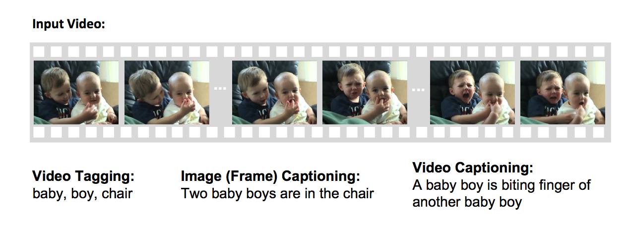
There is also a difference between video tagging and video captioning. Video tagging is to describe what is the video, and it can also extend to where the objects are, while video captioning is trying to use natural sentence to describe what the objects in the videos are interacting to each other, attempting to extract more in-depth meanings from the context of the video.

There is a picture in the original paper explain this very well: tagging vs captioning

Recent development in translation has inspired many good research in the field despite the fact this it is a very difficult problem. In general, CNNs are used to extract visual representation on the videos and RNNs (LSTM) are used to general natural languages.

There are mainly two directions for video captioning: template-based language model, and sequence learning model (RNNs).

The paper also discuss about the research and methodologies to approach the two models and the architectures of a typical video captioning system (section 4.2 - 4.3).

Databases, benchmarks and competitions

The authors also list many useful resources to the problem, mainly databases and competitions.

Some of the databases and competitions are for video classification and some of them are for video captioning.

Order Statistics

|

Order statistic is interesting because it is a little bit different from the often seen probability distributions. The nature of the order statistics allows us to design sampling methods that save us money and time. In certain experiments when there are strict constrains on measurements of samples or the number of samples we can take, order statistic can sometimes help us identify the best model using limited information.

Definition

Supposed we have a random sample with size n associated with random variables \(X_i = \{X_1, X_2, ..., X_n\}\) and each from the a continuous distribution \(f(x)\), then the joint pdf can be derived as the followings:

[f(x_1,x_2,…,x_n) = f(x_1)f(x_2)…f(x_n)]

If we order these random samples from the smallest to the largest and name them \(x_{1:n}, x_{2:n}, ..., x_{n:n}\), we get a list of numbers in order, where the smallest number is \(x_{1:n}\) and the largest number is \(x_{n:n}\).

Now we define a set of new random variables, \(Y_{i} = \{Y_1, Y_2, ...,Y_n\}\), where \(y_{1} = x_{1:n}, y_{2} = x_{2:n}, ..., y_{n} = x_{n:n}\). From this definition we can see that each random variable in \(Y_{i}\) is actually a function of the n random variables from \(X_{i}\), where:

[\begin{array}{lcl} y_1=u_1(x_1,x_2,…,x_n) & = & \min(x_1,x_2,…,x_n)
y_i=u_k(x_1,x_2,…,x_n) & = & i_{th}\min(x_1,x_2,…,x_n)
y_n=u_n(x_1,x_2,…,x_n) & = & \max(x_1,x_2,…,x_n) \end{array}]

We called this set of ordered random variables \(Y_i\) order statistics.

The joint pdf of \(Y_1, Y_2,...,Y_n\)

Then we can derive the joint distribution of \(Y_{i}=\{Y_1, Y_2,...,Y_n\}\) by the following equation:

[g(y_1,y_2,…,y_n)=n!f(y_1)f(y_2)…f(y_n), y_1<y_2<…<y_n]

The intuition of the equation is that if we have a list of unordered samples \(y_1=x_{1:n}, y_2=x_{2:n},...,y_n=x_{n:n}\), the probability of them appearing at the same time in a particular order is \(f(y_1)f(y_2)...f(y_n)\), and we have \(n!\) ways of ordering these random samples. For all different orderings they all have the same order statistics, because they are the same when we order them from the smallest to the largest.

The pdf of the \(k_{th}\) order statistic \(Y_{k}\)

Using integration techniques over all other random variables except \(y_k\) from \(g(y_1,y_2,...,y_n)\), we get:

[g_k(y_k) = \frac{n!}{(k-1)!(n-k)!}[F(y_k)]^{k-1}[1-F(y_{k})]^{n-k}f(y_k)]

Where \(F(x_{i})\) is the CDF of \(X_i\). The intuition is that \(P(X_{i}<=y_k)\) is \(F(y_k)\) and there are \((k-1)\) of samples smaller than \(y_k\), while \(P(X_{i}>=y_k)\) is \((1-F(y_k))\) and there are (n-k) samples greater than \(y_k\). Similar to the way we think about the joint pdf of \(Y_{i}\), we get the pdf of the kth order statistic.

From the kth order statistic distribution we can derive the distribution of \(Y_{1}\) and \(Y_{n}\):

[\begin{array}{l} g_1(y_1)=n[1-F(y_1)]^{n-1}f(y_1)
g_n(y_n)=n[F(y_n)]^{n-1}f(y_n) \end{array}]

The CDF of \(Y_k\)

From the pdf of \(g_1(y_1)\) and \(g_n(y_n)\) we can derive the CDF of them \(G_1(y_1)\) and \(G_n(y_n)\).

[\begin{array}{lcl} G_1(y_1)&=&P[Y_1\leq y_1]
&=&1-P[Y_1>y_1]
&=&1-P[(X_1>y_1)\cap(X_2>y_1)\cap…\cap(X_n>y_1)]
&=&1-[1-F(y_1)]^n \end{array}]

The intuition of \(G_1(y_1)\) is that the probability of the smallest number of all random samples from \(X_i\) is smaller than or equal to \(y_1\), which is equal to the probability of all the samples in \(X_i\) are greater than \(y_i\).

[\begin{array}{lcl} G_n(y_n)&=&P[Y_n\leq y_n]
&=&P[(X_1<y_1)\cap(X_2<y_1)\cap…\cap(X_n<y_1)]
&=&[F(y_n)]^n \end{array}]

The intuition of \(G_1(y_1)\) is that the probability of the largest number of all random samples from \(X_i\) is smaller than or equal to \(y_1\), which is equal to the probability of all samples from \(X_i\) are smaller than or equal to \(y_1\).

Similarly, we can derive the CDF of \(Y_k\):

[\begin{array}{lcl} G_k(y_k)&=&P[Y_k\leq y_k] \end{array}]

Since \(P[Y_k\leq y_k]\) is the probability of the kth order \(Y_k\) is smaller than \(y_k\) and \(Y_k = X_{k:n}\), we get \(P[Y_k\leq y_k] = P[X_{k:n}\leq y_k]\). It means that we need to have at least k number of samples from \(X_{i}\) that are smaller \(y_k\).

From the CDF of \(X_{i}\) we know that \(P[X_{i}<=y_{k}] = F(y_k)\). Now we define a random variable \(K\), which is the number of the \(n\) samples smaller than \(y_k\). The distribution of \(K\) is a binomial distribution with pdf:

[bin(k;n, p) = {n \choose k}p^k(1-p)^{n-k}]

where \(p=P[X_{i}<=y_k]=F(y_k)\).

Then we can calculate the probability of at least \(k\) number of \(X_i\) are smaller than \(y_k\), \(P[K>=k]\), by following the CDF of bin(k;n,p):

[\begin{array}{lcl} P[K>=k]&=&1-P[K<k]
&=&1 - \sum_{j=0}^{k-1}bin(j;n,p)
&=&\sum_{j=k}^{n}bin(j;n,p)
&=&\sum_{j=k}^{n}{n \choose j}[F(y_k)]^j[1-F(y_k)]^{n-j} \end{array}]

Then we can conclude that:

[\begin{array}{lcl} G_k(y_k)&=&P[Y_k\leq y_k]\&=&P[K>=k]\&=&\sum_{j=k}^{n}{n \choose j}[F(y_k)]^j[1-F(y_k)]^{n-j}\end{array}]

Application

One example of using order statistic is Type I and Type II censored sampling. These sampling methods are developed to handle some situations where it is impossible to have complete information about the entire sample. In these cases, if we want to derive a statistical model from the observed data, these sampling techniques can help us develop the joint pdfs that allow us to evaluate our model under some physical constrains.

Type II censored sampling: with a random sample size of n, we stop the experiment after achieving the first r desired outcomes. The marginal density function of the first r order statistics is given by:

[g(y_1, y_2, …, y_r) = \frac{n!}{(n-r)!}[1-F(y_r)]^{n-1}\prod_{i=1}^{r}f(y_i)]

if \(-\infty < y_1 < ... < y_r < \infty\) and zero otherwise.

Some experiments such as measuring the lifetime a certain product, waiting the entire sample to die out and measure all of their life time is too time consuming. A lot of the times, only a portion of the samples (eg. the life time of the first r ordered samples) are measured and a joint pdf of the ordered statistic can be derived by the above formula.

Type I censored sampling: instead of terminating the experiment after achieving a certain number desired outcomes, Type I censored sample terminate the experiment whenever \(Y\) hits a preset value.

For example, in the lifetime experiment of a product mentioned in Type II censored sampling, we might decide to terminate the experiment when \(Y\) is at time \(t_{0}\) and record the lifetime the die out products as \(Y_i=\{Y_1,...,Y_{r}\}\).

The joint pdf of \(Y_{1},...,Y_{r}\) is given by:

[f_{Y_1,…,Y_R}(y_1,…,y_r)=\frac{n!}{(n-r)!}[1-F(t_{0})]^{n-r}\prod_{i=1}^{r}f(y_i)]

if \(y_1 <...< y_r < t_0\) and \(r=1,2,...,n\).

Reference:

All the above formulas and writings are summarized from a classic book Introduction to Probability and Mathematical Statistics by Bain/Engelhardt.

Study Notes - Deep Learning for Video Classification and Captioning (1)

|

This blog post is a study note summary for the paper Deep Learning for Video Classification and Captioning published by Zuxuan Wu, Ting Yao, Yuanwei Fu, and Yu-Guang Jiang in 2016.

This paper provides a great introduction and review of the research on video classification and video captioning. It is a very good first read for researchers who are new to the video processing and natural language processing with some machine learning and deep learning background.

Problem

With the availability of video data, a need has raised to develop applications to understand the meaning of video streams. Video captioning and video classification are two main lines of research to this problem. This paper is a review of resent research on the two topics with an emphasis on deep learning and feature extraction.

Deep Learning Modules

  • Convolutional Neural Networks (CNNs)
    • LeNet-5: back-prop, end-to-end
    • Deep Brief Network: greedy? train each layer in an unsupervised manner
    • AlexNet: 5 conv layers + 3 fully connected layers, RuLU, Dropout
    • VGGNet: 16-19 layers, 3x3 conv filters, able to capture details of input
    • GoogLeNet: multi-scale processing, 22 layers, inception
    • ResNet: 152 - 1000 layers
    • Trend: increasing depth
  • Recurrent Neural Networks (RNNs)
    • Good for sequence labeling (speech, sentence, words)
    • cyclicle connection to form cycle, memory
    • unable to carry long-range dependencies
    • vanishing and exploding gradient problems
  • Long Short-term Memory (LSTM)
    • store and access information in a long run sequence

Video Classification

Classify video streams into different categories, for example, human activities.

  • Image-based video Classification
    • video treated as a collection of frames
    • each frame feed in pre-trained start-of-the-art deep models (AlexNet, GoogLeNet, etc.) till a certain fully connected layer
    • average the output and feed into a standard classifier such as SVM
  • End-to-end CNN Architecture
    • learn hidden spatial-temporal patterns
    • 3D CNN - not performing well because lack of large labeled training data and training is slow
    • 2D CNN - two-stream approach, break the image down in to spatial and temporal clues, Trajectory-Pooled Descriptors - alot of other approaches
  • Modeling Long-Term Temporal Dynamics
    • The two stream approach does not take into account the order of of the video stream since the input is taking in frame by frame
    • Leverage RNN (LSTM)
    • LSTM and CNN are highly complementary
  • Incorporating Visual Attention
    • detect useful and relevant frames
    • attention mechanism to identify the most discriminative spatial-temporal volumes
    • Motion based Attention
  • Unsupervised Video Feature Learning
    • Challenge - not enough training data
    • Use unsupervised learning to find video patterns