
Stanford UFLDL Tutorial Work Through (2) - Logistic Regression
18 Jun 2017 | Deep LearningLink to the tutorial: Unsupervised Feature Learning and Deep Learning: Logistic Regression
Problem
To illustrate logistic regression, let’s reuse the notation of the variables \(X\), \(\Theta\), and \(Y\) from section (1) for linear regression.
Different from linear regression, which is usually used to predict continuous output values, logistic regression is used in classification problems, which have discrete \(y\) outputs. For example, in a two class classification problem, the \(y\) output has two values, 0 and 1. In a logistic regression problem, we want to find a function \(H_{\Theta}\) such that \(H_{\Theta}(X)\) produces a output vector that matches as much as possible to the output variable \(Y\).
Sigmoid/Logistic Function
Before we derive the cost function of logistic regression, we need to introduce a convenient function called the sigmoid function, or logistic function if you like. The function is given by:
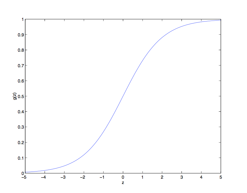
\[S(z)=\frac{1}{1+e^{-z}}\]The sigmoid function has the following properties:
- It is a “S” shape function bounded between 0 and 1. This is usefully because in the process of generating a binary output from \(H_{\Theta}(X)\), the sigmoid function is used to convert the output of a linear function, say \(Z = X\Theta\), into a probability that is used in calculate the cost. Please find the the graph of the sigmoid function below:
- The derivative of the sigmoid function has a very nice form that makes logistic regression a very clean linear method. The derivative is given in the following:
The maximum likelihood function \(\ell(\Theta)\)
Now we can define the following two functions to calculate the probabilities an input record belongs to a certain class:
\[\begin{array}{l} P(y=1|x^{(i)})=h_{\Theta}(x^{(i)})=S(x^{(i)}\Theta)=\frac{1}{1+e^{-x^{(i)}\Theta}}\\ P(y=0|x^{(i)})=1-P(y=1|x^{(i)})=1-h_{\Theta}(x^{(i)})\end{array}\]Note that the above two probability expressions can be combined into one:
\[P(y|x^{(i)})=(h_{\Theta}(x^{(i)}))^y(1-h_{\Theta}(x^{(i)}))^{1-y}\]Then we can derived a log likelihood function for parameter \(\Theta\) using all the input records \(X\) and output variable \(Y\):
\[\begin{array}{ccl} \ell(\Theta)&=&ln[L(\Theta)]\\ &=&ln[\prod_{i=1}^m P(y_i|x^{(i)})]\\ &=&ln[\prod_{i=1}^m (h_{\Theta}(x^{(i)}))^{y_i}(1-h_{\Theta}(x^{(i)}))^{1-{y_i}}]\\ &=&\sum_{i=1}^m [y_iln(h_{\Theta}(x^{(i)}))+(1-y_i)ln(1-h_{\Theta}(x^{(i)}))] \end{array}\]We maximize the log likelihood function by using gradient descent. Similar to what we did in the linear regression lesson, we first calculate the gradient of the maximum likelihood function:
\[\begin{array}{ccl} \frac{\partial \ell(\Theta)}{\partial \theta_j}&=&\frac{\partial}{\partial \theta_j}\sum_{i=1}^m [y_iln(h_{\Theta}(x^{(i)}))+(1-y_i)ln(1-h_{\Theta}(x^{(i)}))]\\ &=&\frac{\partial}{\partial \theta_j}\sum_{i=1}^m [y_iln(S(x^{(i)}\Theta))+(1-y_i)ln(1-S(x^{(i)}\Theta))]\\ &=&\sum_{i=1}^m \frac{\partial}{\partial \theta_j}[y_iln(S(x^{(i)}\Theta))+(1-y_i)ln(1-S(x^{(i)}\Theta))]\\ &=&\sum_{i=1}^m [(y_i\cdot\frac{1}{S(x^{(i)}\Theta)}-(1-y_i)\cdot \frac{1}{1-S(x^{(i)}\Theta)})\cdot \frac{\partial}{\partial \theta_j}S(x^{(i)}\Theta)]\\ &=&\sum_{i=1}^m [(y_i\cdot\frac{1}{S(x^{(i)}\Theta)}-(1-y_i)\cdot \frac{1}{1-S(x^{(i)}\Theta)})\cdot S(x^{(i)}\Theta)\cdot (1-S(x^{(i)}\Theta)\cdot \frac{\partial}{\partial \theta_j}S(x^{(i)}\Theta)]\\ &=&\sum_{i=1}^m [(y_i\cdot(1-S(x^{(i)}\Theta))-(1-y_i)\cdot S(x^{(i)}\Theta))\cdot x_j^{(i)}]\\ &=&\sum_{i=1}^m [(y_i-S(x^{(i)}\Theta))\cdot x_j^{(i)}]\\ &=&X_j^T(Y-H_{\Theta}(X)) \end{array}\]Therefore, the gradient of the log likelihood function is:
\[\nabla \ell_{\Theta}(\Theta)=\left( \begin{array}{c} \frac{\partial {\ell(\Theta)}}{\partial\theta_0}\\ \frac{\partial {\ell(\Theta)}}{\partial\theta_1}\\ \vdots\\ \frac{\partial {\ell(\Theta)}}{\partial\theta_n} \end{array} \right)=X(Y-H_{\Theta}(X))\]We then randomly initialize the \(\Theta\) and iteratively look for the local maximum of \(\ell(\Theta)\) by updating \(\Theta\) in each iteration with \(\Theta:=\Theta+\alpha\nabla \ell_{\Theta}(\Theta)\).
Exercise 2 Solution
Please see this github repo for the solution to exercise 2.
Comments